Fitting geometry through source visibility

This tutorial fits the position and shape of a blue polygon in front of a textured plane. The polygon determines which image features can be sampled onto the plane. When its boundary is in the wrong place, some samples contain the polygon’s color and others discard visible texture. A loss on these samples can move the occluding geometry into place.

The fit starts from a smaller, displaced polygon. White dots mark its boundary vertices; the dashed contour marks the target. The camera and error color scale stay fixed. The curve compares the fit with a run that disables boundary gradients, starting from the same mesh.

Scene and supervision

The scene contains two opaque surfaces: a polygon at camera depth 1 and a plane at depth 2. RGB channels serve as the feature image. The polygon’s center and twenty boundary radii are optimized; its depth and the camera are fixed. Radii at ordered angles keep the boundary connected during fitting.

This synthetic example generates a source image and target sampled features from the target mesh. Those feature values supply supervision for the fit. The rendered comparison panels visualize the geometry; the optimization loss is computed from the samples on the rear plane.

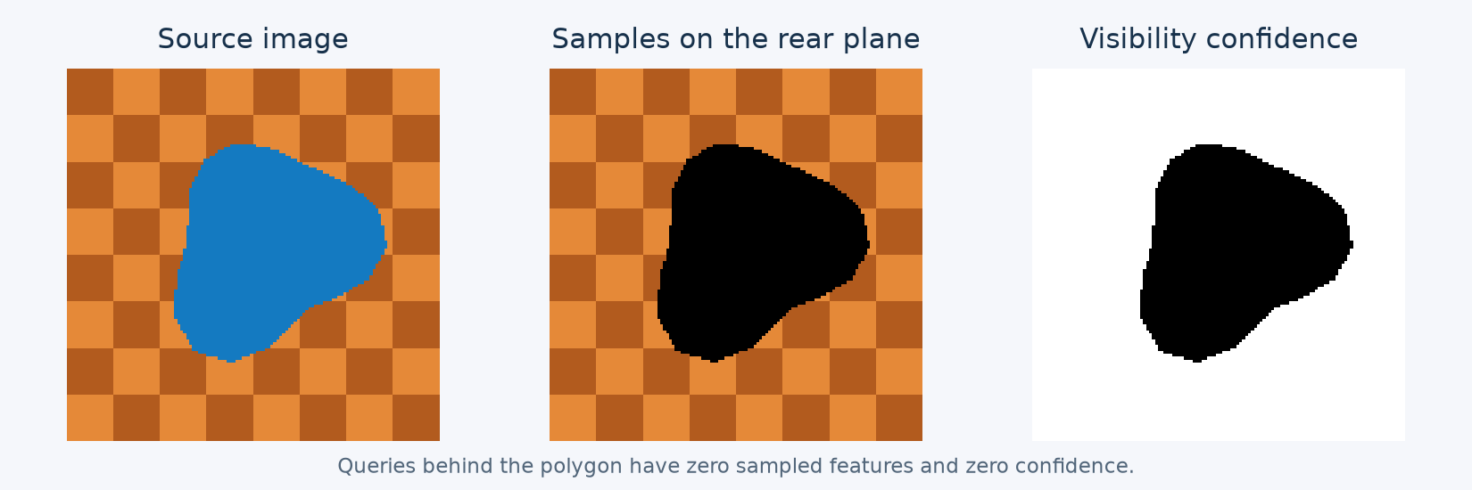
Samples behind the opaque polygon have zero features and zero confidence. Visible samples retain the plane’s texture.

Surface queries

Choose a face and 3D barycentric coordinates for each point where features will be sampled. Here, a regular grid of points lies on the rear plane. Project the mesh vertices into the source camera to obtain pixel XY and positive camera Z.

For a mesh built with drtk.pixel_grid_mesh(), v contains the displaced camera-space positions and uv_anchor gives the original texture coordinates:

v, uv_anchor, uv_reprojected, faces, opacity, _, _ = drtk.pixel_grid_mesh(
    depth, displacement, intrinsics,
    alive, join_right, join_down,
    feather_width=feather_width,
)

A query’s face identifies its local surface. This matters at cuts and shared crack tips, where coincident points may belong to different sides of the mesh.

Sampling

Compute the sampling stencil from the projected geometry, then apply it to the feature image:

indices, weights, source_uv, source_z = drtk.source_feature_stencil(
    v_source_pixels, faces, query_faces, query_barycentrics,
    feature_height, feature_width,
    vertex_opacity=opacity,
    return_queries=True,
)
sampled, confidence = drtk.sample_feature_stencil(
    features, indices, weights
)

sampled has shape (N, C, Q) and confidence has shape (N, 1, Q). The weights combine bilinear interpolation with source transmittance. They also account for image boundaries and the receiving surface’s extent. Additional feature maps with the same batch and image dimensions can use indices and weights from this call.

Fitting the boundary

For sampled features \(S_q(\theta)\) and target samples \(S_q^*\), the example minimizes

\[L(\theta)=\frac{1}{CQ}\sum_{q=1}^{Q} \left\|S_q(\theta)-S_q^*\right\|_2^2,\]

where \(\theta\) contains the polygon’s center and boundary radii. Recompute the stencil after every geometry update:

optimizer.zero_grad()
v_source_pixels = make_vertices(center, radii)
indices, weights, _, _ = drtk.source_feature_stencil(
    v_source_pixels, faces, query_faces, query_barycentrics, H, W
)
sampled, confidence = drtk.sample_feature_stencil(features, indices, weights)
loss = (sampled - target_samples).square().mean()
loss.backward()
optimizer.step()

An opaque polygon’s visibility changes at its boundary. Smooth interpolation derivatives alone do not move this boundary, so the control run stays at its initial shape. DRTK’s boundary-motion estimator supplies the missing geometry gradient. It is enabled by default through edge_gradients=True.

At 128 by 128 pixels, the example reduces sampled-feature MSE by about 97% over 240 Adam steps. A small residual remains near the rasterized boundary. The image does not constrain the polygon’s depth while its ordering is unchanged; this example therefore fits its projected shape.

For topology optimization with drtk.bernoulli_render_loss(), construct the mesh and its stencil inside the loss callback so that each sampled topology has its own visibility.

Combining observations

For applications that update features already stored on a surface, confidence can blend the new observations with existing features:

refined = sampled + (1.0 - confidence) * anchor_features

sampled already includes the visibility weights. Where confidence is zero, the result is entirely the anchor feature. A learned refinement model can instead take anchor features, sampled features, confidence, and geometric context as inputs. Confidence lets it distinguish a missing observation from an observed feature value of zero. The resulting features can be stored on the mesh for rendering from other viewpoints.

Run the example

Download source_features_demo.py. It requires a CUDA-enabled DRTK installation, Matplotlib, and FFmpeg.

python source_features_demo.py --output ./source_features_demo

The output directory contains the comparison figures, an H.264 video, per-step measurements, and saved boundary coordinates. The video records actual optimizer states, with a pause at the beginning and end. See drtk.source_features for argument shapes, coordinate conventions, and gradient behavior.