Simplest Case of Geometry Optimization

In this tutorial, we will see how to setup a minimal example of geomtry optimization.

Imports

import drtk
import torch as th
import torch.nn.functional as thf
from IPython.display import display
from PIL import Image
from torchvision.utils import save_image

I0930 213945.818 _utils_internal.py:314] NCCL_DEBUG env var is set to None
I0930 213945.821 _utils_internal.py:323] NCCL_DEBUG is INFO from /etc/nccl.conf

Triangle Scene

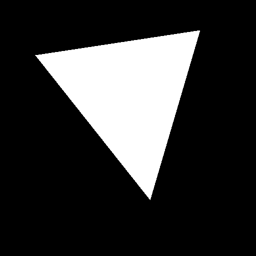
For simplicity, we set up a single triangle without color; only a binary mask will be rendered. Our goal is to optimize this binary mask. For now, we’ll render an image to use as the ground truth.

Next, we’ll modify the vertex positions to new values and attempt to recover the original positions by minimizing the loss between the current mask and the ground truth mask.

v = th.as_tensor(
    [[70, 110, 10], [400, 60, 10], [300, 400, 10]], dtype=th.float32
).cuda()[None]
vi = th.as_tensor([[0, 1, 2]], dtype=th.int32).cuda()

index_img = drtk.rasterize(v, vi, width=512, height=512)

image_gt = (index_img != -1).float()

save_image(image_gt, "img.png")
display(Image.open("img.png"))

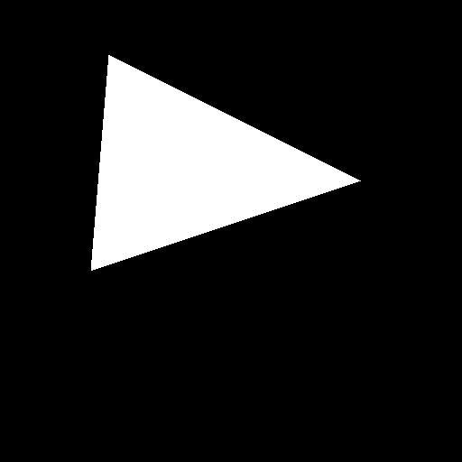
Next, we create a new vertex buffer with updated vertex positions. Let’s render the new mask generated by these positions.

v = th.as_tensor(
    [[120, 60, 10], [400, 200, 10], [100, 300, 10]], dtype=th.float32
).cuda()[None]

index_img = drtk.rasterize(v, vi, width=512, height=512)
depth_img, bary_img = drtk.render(v, vi, index_img)

image = (index_img != -1).float()

save_image(image, "img.png")
display(Image.open("img.png"))

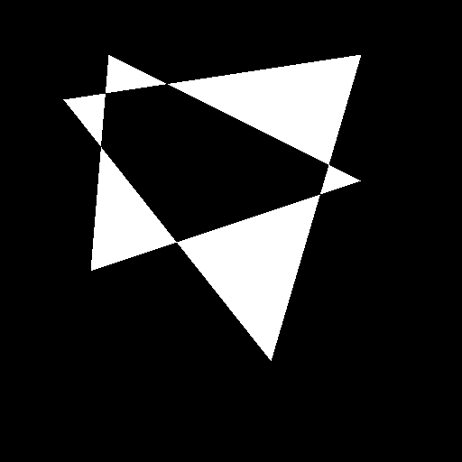
Next, we compute l2 loss. Let’s visualize it.

l2_loss = thf.mse_loss(image, image_gt, reduction="none")

save_image(l2_loss, "img.png")
display(Image.open("img.png"))

Next, we will pass the current rendered mask through edge_grad_estimator to make it differentiable. We will also use a hook in order to visualize the computed gradients per fragment

# Need to make vertex positions differentiable, otherwise the gradient will not be computed.
v.requires_grad_(True)
v.grad = None

tensor = []


# A simple hook to save the gradient
def save_tensor(x: th.Tensor):
    tensor.append(x)


# Make `image` differentiable
image_differentiable = drtk.edge_grad_estimator(
    v, vi, bary_img, image[:, None], index_img, v_pix_img_hook=save_tensor
)

# Compute loss and backpropagate
difference = thf.mse_loss(image_differentiable, image_gt[:, None], reduction="none")
difference.sum().backward()

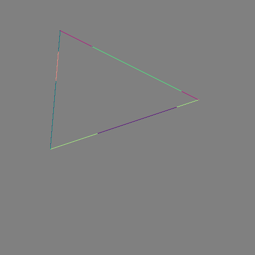
Let’s visualize the saved gradient

save_image(tensor[0].mul(.5).add(0.5), "img.png")
display(Image.open("img.png"))

To better see the details, we can visualize it per component, using a colormap

def conv_img_viridis(x: th.Tensor) -> Image:
    import seaborn as sns
    import numpy as np

    with th.no_grad():
        assert x.ndim == 2
        colored = (
            sns.blend_palette(["#8c179a", "#64c5c2", "#fef46a"], 6, as_cmap=True)(
                x.cpu().numpy().squeeze()
            )[..., :-1]
            * 255.0
        ).astype(np.uint8)
        return Image.fromarray(colored)

X component:

display(conv_img_viridis(tensor[0][0, 0].mul(0.5).add(0.5)))

Y component:

display(conv_img_viridis(tensor[0][0, 1].mul(0.5).add(0.5)))

Z component as expected is zero. Z component can be non-zero only whenocclusion order can change due to the vertex movement.

display(conv_img_viridis(tensor[0][0, 2].mul(0.5).add(0.5)))

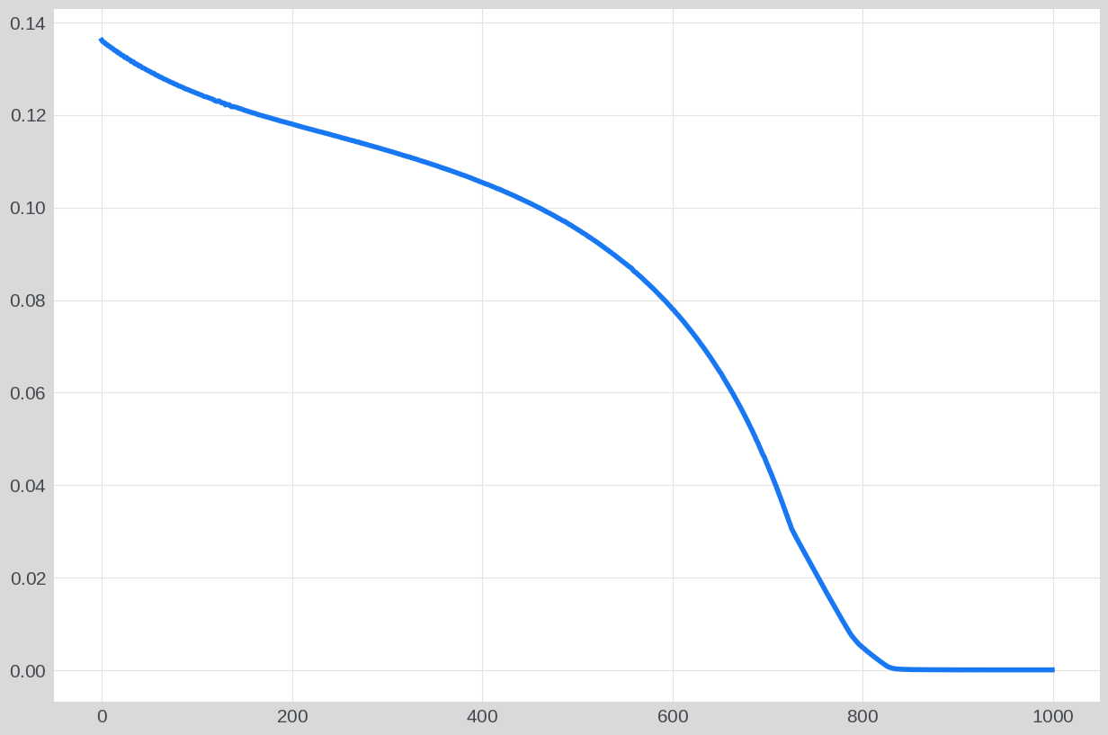
Next, we will try to optimize vertex position:

import matplotlib.pyplot as plt
from tqdm import tqdm

v = th.as_tensor(
    [[120, 60, 10], [400, 200, 10], [100, 300, 10]], dtype=th.float32
).cuda()[None]

v_param = th.nn.Parameter(v)

opt = th.optim.SGD([v_param], lr=1000.0)
loss_list = []


for iter in tqdm(range(1000)):
    tensor.clear()

    index_img = drtk.rasterize(v_param, vi, width=512, height=512)
    depth_img, bary_img = drtk.render(v_param, vi, index_img)

    image = (index_img != -1).float()

    # Make `image` differentiable
    image_differentiable = drtk.edge_grad_estimator(
        v_param, vi, bary_img, image[:, None], index_img, v_pix_img_hook=save_tensor
    )

    # Compute loss and backpropagate
    l2_loss = thf.mse_loss(image_differentiable, image_gt[:, None])
    l2_loss.backward()
    opt.step()
    opt.zero_grad()

    loss_list.append(l2_loss.item())


plt.plot(loss_list)
plt.show()

100%|██████████| 1000/1000 [00:12<00:00, 81.47it/s]

Now, we will rerun the same optimization, but this time, we’ll also save a video showing the current versus target geometry, along with the x and y components of the gradients.

import av
import imageio
import IPython.display
import numpy as np
from PIL import Image, ImageDraw, ImageFont
from tqdm import tqdm

container = av.open(
    "out.mp4",
    mode="w",
    format="mp4",
    options={"movflags": "frag_keyframe+empty_moov"},
)

video_stream = container.add_stream(
    "libx264",
    width=1024,
    height=1024,
    pix_fmt="yuv420p",
    framerate=24,
)
font = ImageFont.truetype("/usr/share/fonts/truetype/ttf-dejavu/DejaVuSans.ttf", 16)

v = th.as_tensor(
    [[120, 60, 10], [400, 200, 10], [100, 300, 10]], dtype=th.float32
).cuda()[None]

v_param = th.nn.Parameter(v)

tensor = []

opt = th.optim.SGD([v_param], lr=1000.0)


# A simple hook to save the gradient
def save_tensor(x: th.Tensor):
    tensor.append(x)


def conv_img(x: th.Tensor) -> th.Tensor:
    with th.no_grad():
        x = (x * 255).type(th.long).clamp(0, 255).cpu()
        if len(x.shape) == 4:
            x = x[0, :, :, :]
        return x.type(th.uint8).transpose(0, 2).transpose(0, 1)


for iter in tqdm(range(1000)):
    tensor.clear()

    index_img = drtk.rasterize(v_param, vi, width=512, height=512)
    depth_img, bary_img = drtk.render(v_param, vi, index_img)

    image = (index_img != -1).float()

    # Make `image` differentiable
    image_differentiable = drtk.edge_grad_estimator(
        v_param, vi, bary_img, image[:, None], index_img, v_pix_img_hook=save_tensor
    )

    # Compute loss and backpropagate
    l2_error = thf.mse_loss(image_differentiable, image_gt[:, None], reduction="none")
    l2_loss = l2_error.mean()
    l2_loss.backward()
    opt.step()
    opt.zero_grad()
    if iter % 16 == 0:
        im = conv_img(image)
        im[:129, :129] = 255
        im[:128, :128] = conv_img(thf.avg_pool2d(image_gt[None, ...], 4))

        error = conv_img(thf.interpolate(l2_error, scale_factor=1.0))
        grad = tensor[0]

        grad = grad * 400000.0
        gimx = th.as_tensor(np.asarray(conv_img_viridis(grad[0, 0] * 0.5 + 0.5)))
        gimy = th.as_tensor(np.asarray(conv_img_viridis(grad[0, 1] * 0.5 + 0.5)))
        im[-1:] = 255
        error[-1:] = 255

        im1 = th.cat([im, error], dim=0)
        im2 = th.cat([gimx.expand(-1, -1, 3), gimy.expand(-1, -1, 3)], dim=0)

        im = th.cat([im1.expand(-1, -1, 3), im2], dim=1)

        im = Image.fromarray(im.cpu().numpy())
        draw = ImageDraw.Draw(im)
        draw.text((0, 128 - 20), " Target", (255, 255, 255), font=font)
        draw.text((0, 512 - 25), " Render", (255, 255, 255), font=font)
        draw.text((0, 512 + 512 - 25), " Error", (255, 255, 255), font=font)
        draw.text((512, 512 - 25), " grad_x", (255, 255, 255), font=font)
        draw.text((512, 512 + 512 - 25), " grad_y", (255, 255, 255), font=font)

        im = np.asarray(im)
        container.mux(
            video_stream.encode(av.VideoFrame.from_ndarray(im, format="rgb24"))
        )

for packet in video_stream.encode():
    container.mux(packet)
container.close()

IPython.display.Video("out.mp4", embed=True, width=256 * 3, height=256 * 3)

100%|██████████| 1000/1000 [00:14<00:00, 66.91it/s]

This concludes the “Simplest Case of Geometry Optimization” tutorial.